Introduction

• The concept of Data Structures is very important in modern computer science. So, in this course, we would examine what data structure is all about and then we briefly look at different data structures being used today.

• 

• What is Data Structure?

• A data structure is a specialized format for organizing, processing, retrieving and storing data. There are several basic and advanced types of data structures, all designed to arrange data to suit a specific purpose. Data structures make it easy for users to access and work with the data they need in appropriate ways. Most importantly, data structures frame the organization of information so that machines and humans can better understand it.

• To maintain proper structures

• To decrease the time

• How are data structures used?

• data structures are used to implement the physical forms of abstract datatypes. Data structures are a crucial part of designing efficient software. They also play a critical role in algorithm design and how those algorithms are used within computer programs.

• Storing data

• Managing resources and services

• ordering & sorting

• indexing

• searching

• scalability

• Characteristics of data structures

• Linear and non-linear

• 

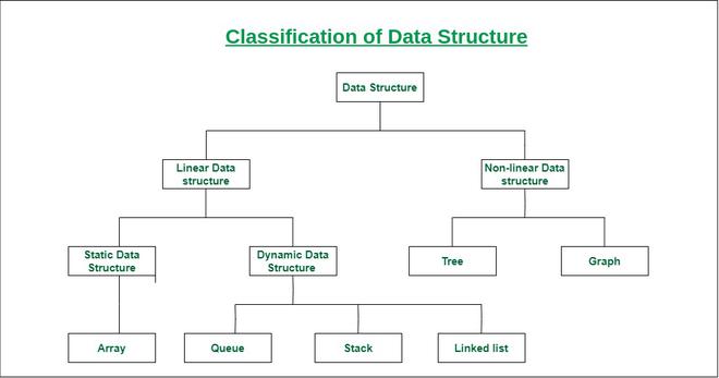
• Homogenous and heterogeneous

• static or dynamic

Linear Data structures:

• Array

• Stack

• Queue

• Linked List - (Single Linked list, Double-liked list)

Non-Linear Data structures:

• Trees - Binary Search Tree

• Graphs

• Heap.

  Arrays:

  An array is a type of data structure that stores multiple data at the same time. An array is a linear data structure that collects elements of the same type of data and stores them in contiguous and contiguous memory locations. Arrays operate in an index system starting from 0 to (n-1), where n is the size of the array.

• It stores the data and access is easy

• array size is fixed.

• Operations of Array:

• sorting

• searching

• Types of arrays-(One-dimensional array. Multi-Dimensional Arrays.)

  

Creating an Array

import array as arr

# creating an array with integer type
a = arr.array('i', [1, 2, 3])

# printing original array
print ("The new created array is : ", end =" ")
for i in range (0, 3):
    print (a[i], end =" ")

Stack :

A stack is an abstract data type that contains an ordered, simple sequence of elements. In contrast to a queue, a stack is a last-in, first-out (LIFO) structure. A real-life example is a stack of books: You can only take a book from the top of the stack and you can only add a book to the top of the stack.

Application of stack:

• Recursion

• Infix and postfix

Operations:

• push - Adding data to the stack

• pop - Removing data from the stack

• peek - accessing the top value of the stack

• display - to print the data in the stack

The stack can be implemented by using

• Arrays

• LinkedList

Stack implementation using Arrays:

class StackUsingArray:
    def __init__(self):
        self.stack = []

    #Method to append the element in the stack at top position.
    def push(self, element):
        self.stack.append(element)

    #Method to Pop last element from the top of the stack
    def pop(self):
        if(not self.isEmpty()):
            lastElement = self.stack[-1] #Save the last element to return
            del(self.stack[-1]) #Remove the last element
            return lastElement
        else:
            return("Stack Already Empty")

    #Method to check if stack is empty or not
    def isEmpty(self):
        return self.stack == []

    def printStack(self):
        print(self.stack)

#Driver code for pro players only :), BTY it is noob friendly.
if __name__ == "__main__":
    s = StackUsingArray()
    print("*"*5+" Stack Using Array HolyCoders.com "+5*"*")
    while(True):
        el = int(input("1 for Push\n2 for Pop\n3 to check if it is Empty\n4 to print Stack\n5 to exit\n"))
        if(el == 1):
            item = input("Enter Element to push in stack\n")
            s.push(item)
        if(el == 2):
            print(s.pop())
        if(el == 3):
            print(s.isEmpty())
        if(el == 4):
            s.printStack()
        if(el == 5):
            break

Stack implementation Using LinkedList:

Instead of using an array, we can also use a linked list to implement a stack. A linked list allocates memory dynamically. However, the time complexity in both scenarios is the same for all operations i.e. push, pop and peek.

In a linked list implementation of a stack, nodes are organized noncontiguous in memory. Each node holds a pointer to its immediate successor node in the stack. A stack overflow is said if there is not enough free space in the memory heap to create a node.

class Node:
    def __init__(self, data):
       self.data = data
       self.next = None

class Stack:
    def __init__(self):
        self.head = None

    def push(self, data):
        if self.head is None:
            self.head = Node(data)
        else:
            new_node = Node(data)
            new_node.next = self.head
            self.head = new_node

    def pop(self):
        if self.head is None:
            return None
        else:
            popped = self.head.data
            self.head = self.head.next
            return popped

a_stack = Stack()
while True:
    print('push <value>')
    print('pop')
    print('quit')
    do = input('What would you like to do? ').split()

    operation = do[0].strip().lower()
    if operation == 'push':
        a_stack.push(int(do[1]))
    elif operation == 'pop':
        popped = a_stack.pop()
        if popped is None:
            print('Stack is empty.')
        else:
            print('Popped value: ', int(popped))
    elif operation == 'quit':
        break

Queue:

A queue is an abstract data structure similar to stacks. Unlike stacks, the queue is open at both ends. One end is always used to insert data (enqueue) and the other is used to remove data (dequeue). The queue follows a first-in-first-out methodology, i.e., the data item stored first is accessed first.

Queue implementation Using Array:

An array implementation of a queue If the sequence is implemented using arrays, the size of the array must be A fixed maximum allowed to expand or shrink a queue. Operations on a Queue have two simple operations.

They are Adding an element to the queue and removing an element from the queue Both variables before and after are used to represent the ends. Front Removes the front end of the queue Happens and the back points to the back end of the queue, here 54 Addition of elements takes place. Initially, when the queue is full, the Front and back are equal to -1.

# Queue implementation in Python

class Queue:

    def __init__(self):
        self.queue = []

    # Add an element
    def enqueue(self, item):
        self.queue.append(item)

    # Remove an element
    def dequeue(self):
        if len(self.queue) < 1:
            return None
        return self.queue.pop(0)

    # Display  the queue
    def display(self):
        print(self.queue)

    def size(self):
        return len(self.queue)


q = Queue()
q.enqueue(1)
q.enqueue(2)
q.enqueue(3)
q.enqueue(4)
q.enqueue(5)

q.display()

q.dequeue()

print("After removing an element")
q.display()

Queue implementation Using LinkedList:

First in First out

1) Enqueue -> inserting an element to the queue

2) Dequeue -> removing element from the queue

3) peek -> to print the first element in the queue

4) display: print all the elements in the queue

# A Linked List Node
class Node:
    def __init__(self, data, left=None, right=None):
        # set data in the allocated node and return it
        self.data = data
        self.next = None


class Queue:
    def __init__(self):
        self.rear = None
        self.front = None
        self.count = 0

    # Utility function to dequeue the front element
    def dequeue(self):          # delete at the beginning
        if self.front is None:
            print('Queue Underflow')
            exit(-1)

        temp = self.front
        print('Removing…', temp.data)

        # advance front to the next node
        self.front = self.front.next

        # if the list becomes empty
        if self.front is None:
            self.rear = None

        # decrease the node's count by 1
        self.count -= 1

        # return the removed item
        return temp.data

    # Utility function to add an item to the queue
    def enqueue(self, item):    # insertion at the end
        # allocate the node in a heap
        node = Node(item)
        print('Inserting…', item)

        # special case: queue was empty
        if self.front is None:
            # initialize both front and rear
            self.front = node
            self.rear = node
        else:
            # update rear
            self.rear.next = node
            self.rear = node

        # increase the node's count by 1
        self.count += 1

    # Utility function to return the top element in a queue
    def peek(self):
        # check for an empty queue
        if self.front:
            return self.front.data
        else:
            exit(-1)

    # Utility function to check if the queue is empty or not
    def isEmpty(self):
        return self.rear is None and self.front is None

    # Function to return the size of the queue
    def size(self):
        return self.count


if __name__ == '__main__':

    q = Queue()
    q.enqueue(1)
    q.enqueue(2)
    q.enqueue(3)
    q.enqueue(4)

    print('The front element is', q.peek())

    q.dequeue()
    q.dequeue()
    q.dequeue()
    q.dequeue()

    if q.isEmpty():
        print('The queue is empty')
    else:
        print('The queue is not empty')

Introduction to Linked List:

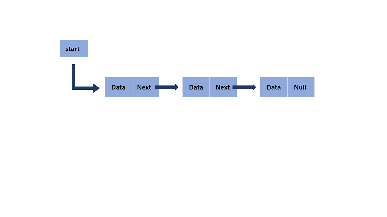
A linked list is a linear data structure that includes a series of connected nodes. Here, each node stores the data and the address of the next node

An important concept A linked list can be used in almost every case where a 1D array is used. The first node of a linked list is called the head. The last node of a linked list is called the tail. tail is always null as the next reference because it is the last element. Next always points to the successor node in the list.

Types of linked list

Single-linked list In a singly linked list, a node has only one reference, which stores the address of the next node in the list. We are going to cover that in this article.

1. Start with a single node

1. Let's start with a single node as linking several nodes gives us a complete list. For this, we create a Node class that holds some data and a next single pointer that is used to point to the next Node-type object in the linked list.

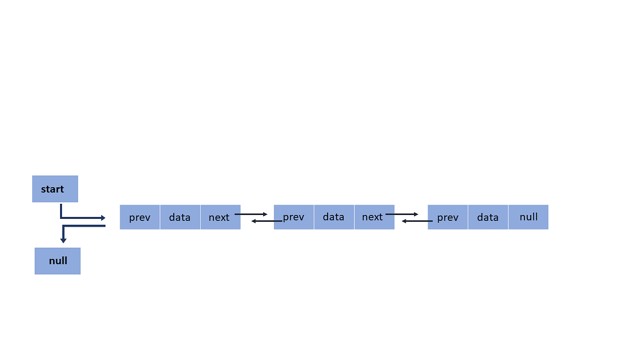
Doubly linked list In a doubly linked list, a node has two references. One to the next node and the other to the previous node.

# A single node of a singly linked list
class Node:
  # constructor
  def __init__(self, data, next=None): 
    self.data = data
    self.next = next

# Creating a single node
first = Node(3)
print(first.data)

2. Join nodes to get a linked list

The next step is to join multiple single nodes that contain data using next pointers and have a single head pointer that points to a complete instance of the linked list.

Using the head pointer, we'll be able to traverse the entire list, even doing all sorts of list manipulations while we're at it.

For this, we create a LinkedList class with a single Head pointer:

# A single node of a singly linked list
class Node:
  # constructor
  def __init__(self, data = None, next=None): 
    self.data = data
    self.next = next

# A Linked List class with a single head node
class LinkedList:
  def __init__(self):  
    self.head = None

# Linked List with a single node
LL = LinkedList()
LL.head = Node(3)
print(LL.head.data)

Add the required methods to the LinkedList class

Last but not least, we can add various linked list manipulation methods to our implementation. Let's look at the insert and print methods for our linked list implementation below:

# A single node of a singly linked list
class Node:
  # constructor
  def __init__(self, data = None, next=None): 
    self.data = data
    self.next = next

# A Linked List class with a single head node
class LinkedList:
  def __init__(self):  
    self.head = None

  # insertion method for the linked list
  def insert(self, data):
    newNode = Node(data)
    if(self.head):
      current = self.head
      while(current.next):
        current = current.next
      current.next = newNode
    else:
      self.head = newNode

  # print method for the linked list
  def printLL(self):
    current = self.head
    while(current):
      print(current.data)
      current = current.next

# Singly Linked List with insertion and print methods
LL = LinkedList()
LL.insert(3)
LL.insert(4)
LL.insert(5)
LL.printLL()

Doubly Linked List

In the Doubly Linked List, the node has two references. One to the next node and another to the previous node

We create a doubly linked list by using the Node class. Now we use the same procedure as in a singly linked list but head and next pointers are used for proper assignment to create two links in each node along with the data in the node.

class Node:
   def __init__(self, data):
      self.data = data
      self.next = None
      self.prev = None

class doubly_linked_list:
   def __init__(self):
      self.head = None

# Adding data elements        
   def push(self, NewVal):
      NewNode = Node(NewVal)
      NewNode.next = self.head
      if self.head is not None:
         self.head.prev = NewNode
      self.head = NewNode

# Print the Doubly Linked list        
   def listprint(self, node):
      while (node is not None):
         print(node.data),
         last = node
         node = node.next

dllist = doubly_linked_list()
dllist.push(12)
dllist.push(8)
dllist.push(62)
dllist.listprint(dllist.head)

Inserting into Doubly Linked List

Here, we are going to see how to insert a node to the Doubly Link List using the following program. The program uses a method named insert which inserts the new node at the third position from the head of the doubly linked list.

# Create the Node class
class Node:
   def __init__(self, data):
      self.data = data
      self.next = None
      self.prev = None

# Create the doubly linked list
class doubly_linked_list:
   def __init__(self):
      self.head = None

# Define the push method to add elements        
   def push(self, NewVal):
      NewNode = Node(NewVal)
      NewNode.next = self.head
      if self.head is not None:
         self.head.prev = NewNode
      self.head = NewNode

# Define the insert method to insert the element        
   def insert(self, prev_node, NewVal):
      if prev_node is None:
         return
      NewNode = Node(NewVal)
      NewNode.next = prev_node.next
      prev_node.next = NewNode
      NewNode.prev = prev_node
      if NewNode.next is not None:
         NewNode.next.prev = NewNode

# Define the method to print the linked list 
   def listprint(self, node):
      while (node is not None):
         print(node.data),
         last = node
         node = node.next

dllist = doubly_linked_list()
dllist.push(12)
dllist.push(8)
dllist.push(62)
dllist.insert(dllist.head.next, 13)
dllist.listprint(dllist.head)

Appending to a Doubly linked list

Appending to a doubly linked list will add the element at the end.

# Create the node class
class Node:
   def __init__(self, data):
      self.data = data
      self.next = None
      self.prev = None
# Create the doubly linked list class
class doubly_linked_list:
   def __init__(self):
      self.head = None

# Define the push method to add elements at the begining
   def push(self, NewVal):
      NewNode = Node(NewVal)
      NewNode.next = self.head
      if self.head is not None:
         self.head.prev = NewNode
      self.head = NewNode

# Define the append method to add elements at the end
   def append(self, NewVal):
      NewNode = Node(NewVal)
      NewNode.next = None
      if self.head is None:
         NewNode.prev = None
         self.head = NewNode
         return
      last = self.head
      while (last.next is not None):
         last = last.next
      last.next = NewNode
      NewNode.prev = last
      return

# Define the method to print
   def listprint(self, node):
      while (node is not None):
         print(node.data),
         last = node
         node = node.next

dllist = doubly_linked_list()
dllist.push(12)
dllist.append(9)
dllist.push(8)
dllist.push(62)
dllist.append(45)
dllist.listprint(dllist.head)

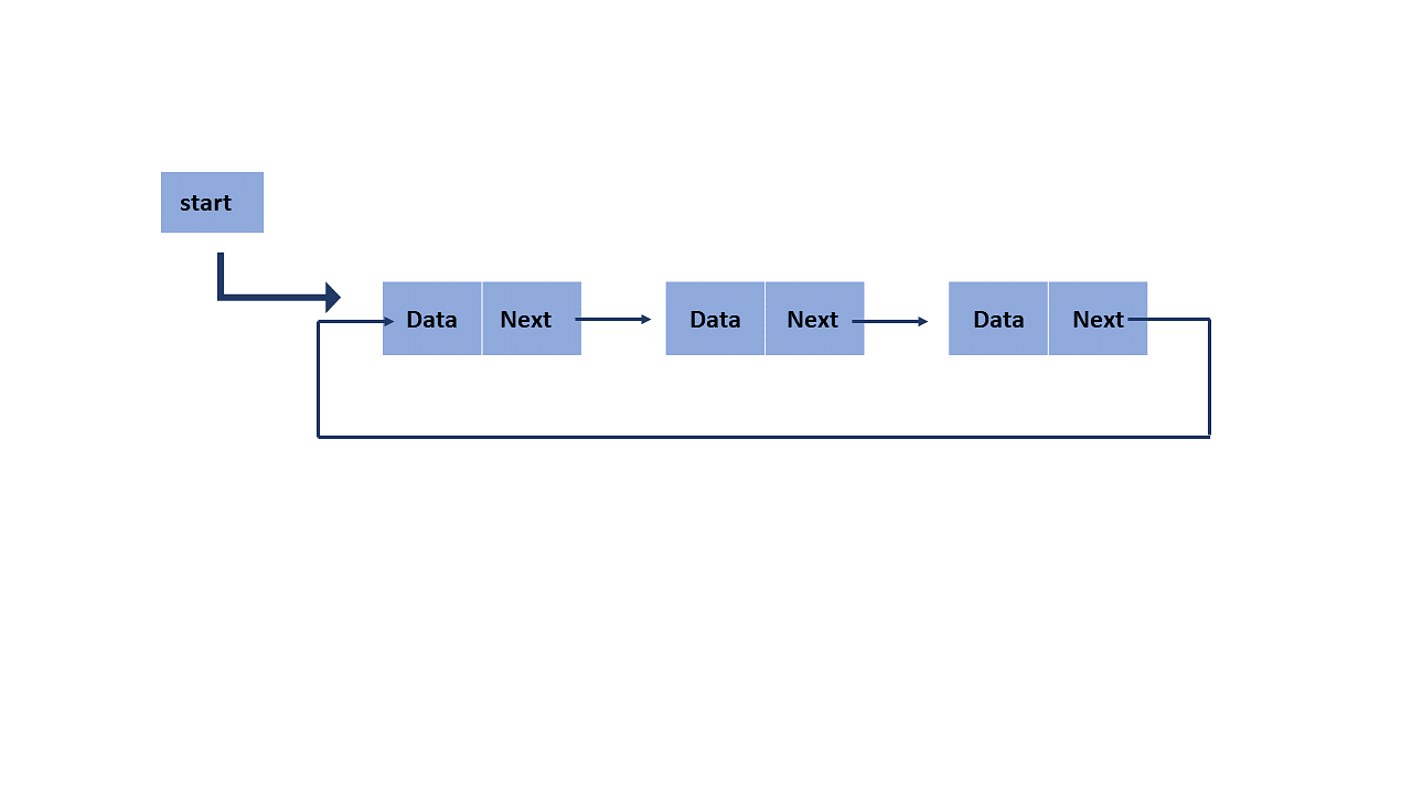
Circular Linked List"

Circular Linked List In a circular linked list, a node can have one or two references. But the tail is connected to the head of the linked list.

Here, the single node is represented as

struct Node {
    int data;
    struct Node * next;
};

Each struct node has a data item and a pointer to the next struct node.

Now we will create a simple circular linked list with three items to understand how this works.

/* Initialize nodes */
struct node *last;
struct node *one = NULL;
struct node *two = NULL;
struct node *three = NULL;

/* Allocate memory */
one = malloc(sizeof(struct node));
two = malloc(sizeof(struct node));
three = malloc(sizeof(struct node));

/* Assign data values */
one->data = 1;
two->data = 2;
three->data = 3;

/* Connect nodes */
one->next = two;
two->next = three;
three->next = one;

/* Save address of third node in last */
last = three;

Applications of Linked List

1. Linked List is heavily used to create stacks and queues.

2. When you need constant-time insertions or deletions from the list.

3. When the size of the list is unknown. This means you don't know how much your list is going to be scaled, then use Linked List instead of Arrays.

4. To implement Hash Tables, Trees or Graphs

Advantages of Linked List

1. Using linked list efficient memory utilization can be achieved since the size of the linked list can be changed at the run time.

2. Stacks and queues are often easily implemented using a linked list.

3. Insertion and deletion are quite easier in the linked list.

Disadvantages of Linked List

1. More memory is required in the linked list compared to an array.

2. Traversal in the linked list is more time-consuming.

3. In a singly linked list reverse traversing is not possible, but it can be done using a doubly linked list which will take even more memory.

4. Random access is not possible due to its dynamic memory allocation.

Trees:

A tree is a non-linear data structure and a hierarchy of collections of nodes, such that each node of the tree stores a value and a list of references to other nodes Children. This data structure is a special way to organize and store data in a computer for more efficient use.

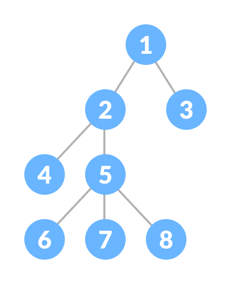
Components of a tree data structure A tree consists of a root node, leaf nodes and internal nodes. Each node is connected to its node by a reference, called an edge.

Root Node: The root node is the top node of the tree. It is always the first node created while creating a tree and we can access each element of the tree starting from the root node. In the example above, the node containing element 50 is the root node.

Parent Node: The parent of any node is the node that refers to the current node. In the example above, 50 is the parent of 20 and 45, and 20 is the parent of 11, 46 and 15. Similarly, 45 is the parent of 30 and 78.

Child Node: The child nodes of the parent node are the nodes that the parent node refers to using references. In the example above, 20 and 45 are children of 50. Nodes 11, 46 and 15 are 20 and 30 and 78 are children of 45.

Edge: A reference to which a parent node is connected to a child node is called an edge. In the above example, every arrow connecting any two nodes is an edge.

Leaf Node: These are the nodes in the tree that have no children. In the above example, 11, 46, 15, 30 and 78 are leaf nodes.

Internal Nodes: Nodes that have at least one child are called internal nodes. In the above example, 50, 20 and 45 are internal nodes.

What is a Binary Tree?

A binary search tree is a data structure that allows us to quickly manage a sorted list of numbers.

It is called a binary tree because each tree node has at most two children. It is called a search tree because it can be used to search for the existence of a number in O(log(n)) time. Characteristics that distinguish a binary search tree from a normal binary tree

All nodes of the left subtree are less than the root node All nodes of the right subtree are greater than the root node Both subtrees of each node are also BSTs i.e. they have the above two properties

Search Operation

The algorithm depends on the property of BST that if each left subtree has values below the root and each right subtree has values above the root.

If the value is below the root, we can say for sure that the value is not in the right subtree; we need to only search in the left subtree and if the value is above the root, we can say for sure that the value is not in the left subtree; we need to only search in the right subtree.

 If root == NULL 
    return NULL;
If number == root->data 
    return root->data;
If number < root->data 
    return search(root->left)
If number > root->data 
    return search(root->right)

Insert operation:

Inserting a value in the correct position is similar to a search, as we try to maintain the rule that the left subtree is less than the root and the right subtree is greater than the root.

We keep going to the right subtree or the left subtree depending on the value and when the left or right subtree reaches a null point, we place a new node there.

If node == NULL 
    return createNode(data)
if (data < node->data)
    node->left  = insert(node->left, data);
else if (data > node->data)
    node->right = insert(node->right, data);  
return node;

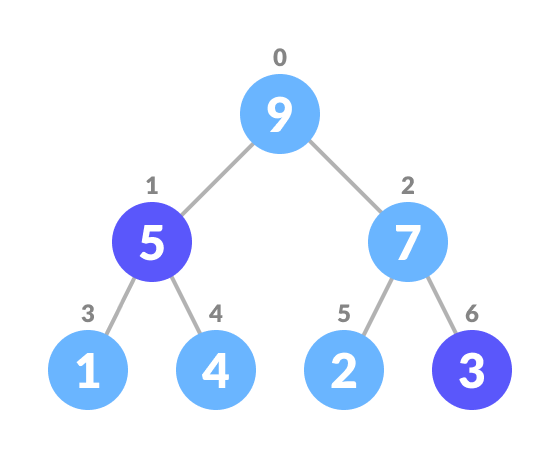
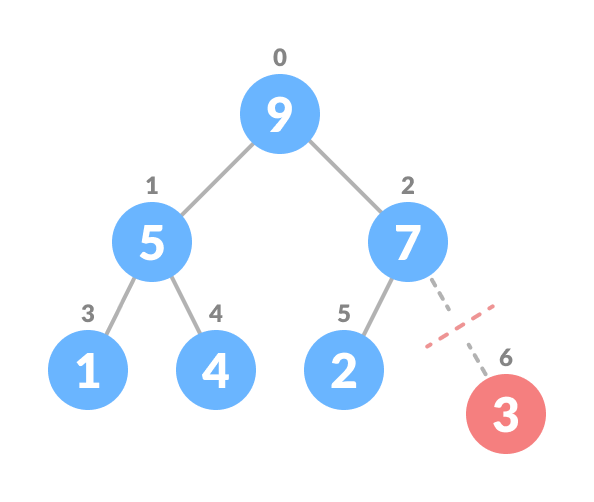
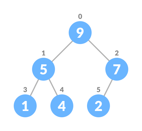
Deletion Operation

There are three cases for deleting a node from a binary search tree.

Case I

In the first case, the node to be deleted is the leaf node. In such a case, simply delete the node from the tree.

Case II

In the second case, the node to be deleted lies has a single child node. In such a case follow the steps below:

1. Replace that node with its child node.

2. Remove the child node from its original position.

Case III

In the third case, the node to be deleted has two children. In such a case follow the steps below:

1. Get the in-order successor of that node.

2. Replace the node with the in-order successor.

3. Remove the in-order successor from its original position.

# Binary Search Tree operations in Python


# Create a node
class Node:
    def __init__(self, key):
        self.key = key
        self.left = None
        self.right = None


# Inorder traversal
def inorder(root):
    if root is not None:
        # Traverse left
        inorder(root.left)

        # Traverse root
        print(str(root.key) + "->", end=' ')

        # Traverse right
        inorder(root.right)


# Insert a node
def insert(node, key):

    # Return a new node if the tree is empty
    if node is None:
        return Node(key)

    # Traverse to the right place and insert the node
    if key < node.key:
        node.left = insert(node.left, key)
    else:
        node.right = insert(node.right, key)

    return node


# Find the inorder successor
def minValueNode(node):
    current = node

    # Find the leftmost leaf
    while(current.left is not None):
        current = current.left

    return current


# Deleting a node
def deleteNode(root, key):

    # Return if the tree is empty
    if root is None:
        return root

    # Find the node to be deleted
    if key < root.key:
        root.left = deleteNode(root.left, key)
    elif(key > root.key):
        root.right = deleteNode(root.right, key)
    else:
        # If the node is with only one child or no child
        if root.left is None:
            temp = root.right
            root = None
            return temp

        elif root.right is None:
            temp = root.left
            root = None
            return temp

        # If the node has two children,
        # place the inorder successor in position of the node to be deleted
        temp = minValueNode(root.right)

        root.key = temp.key

        # Delete the inorder successor
        root.right = deleteNode(root.right, temp.key)

    return root


root = None
root = insert(root, 8)
root = insert(root, 3)
root = insert(root, 1)
root = insert(root, 6)
root = insert(root, 7)
root = insert(root, 10)
root = insert(root, 14)
root = insert(root, 4)

print("Inorder traversal: ", end=' ')
inorder(root)

print("\nDelete 10")
root = deleteNode(root, 10)
print("Inorder traversal: ", end=' ')
inorder(root)

Binary Search Tree Complexities

Time Complexity

Operation	Best Case Complexity	Average Case Complexity	Worst Case Complexity
Search	O(log n)	O(log n)	O(n)
Insertion	O(log n)	O(log n)	O(n)
Deletion	O(log n)	O(log n)	O(n)

Space Complexity

The space complexity for all the operations is O(n).

Graphs :

A graph data structure is a collection of nodes that have data and are connected to other nodes.

Let's try to understand this through an example. On Instagram, everything is a node. That includes User, Photo, Album, Event, Group, Page, Comment, Story, Video, Link, Note...anything that has data is a node.

Every relationship is an edge from one node to another. Whether you post a photo, join a group, like a page, etc., a new edge is created for that relationship.

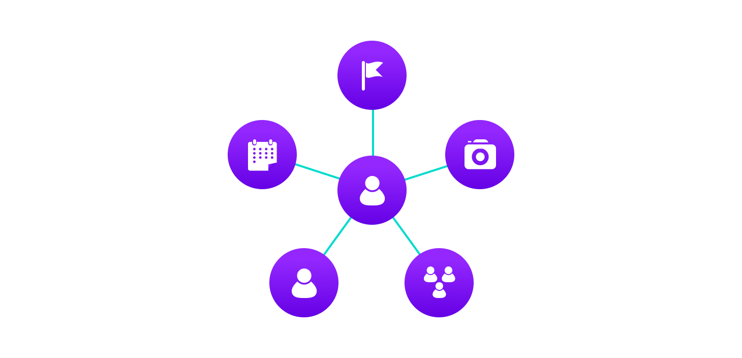
Example of graph data structure

All of Instagram is then a collection of these nodes and edges. This is because Instagram uses a graph data structure to store its data.

More precisely, a graph is a data structure (V, E) that consists of

• A collection of vertices V

• A collection of edges E represented as ordered pairs of vertices (u,v)

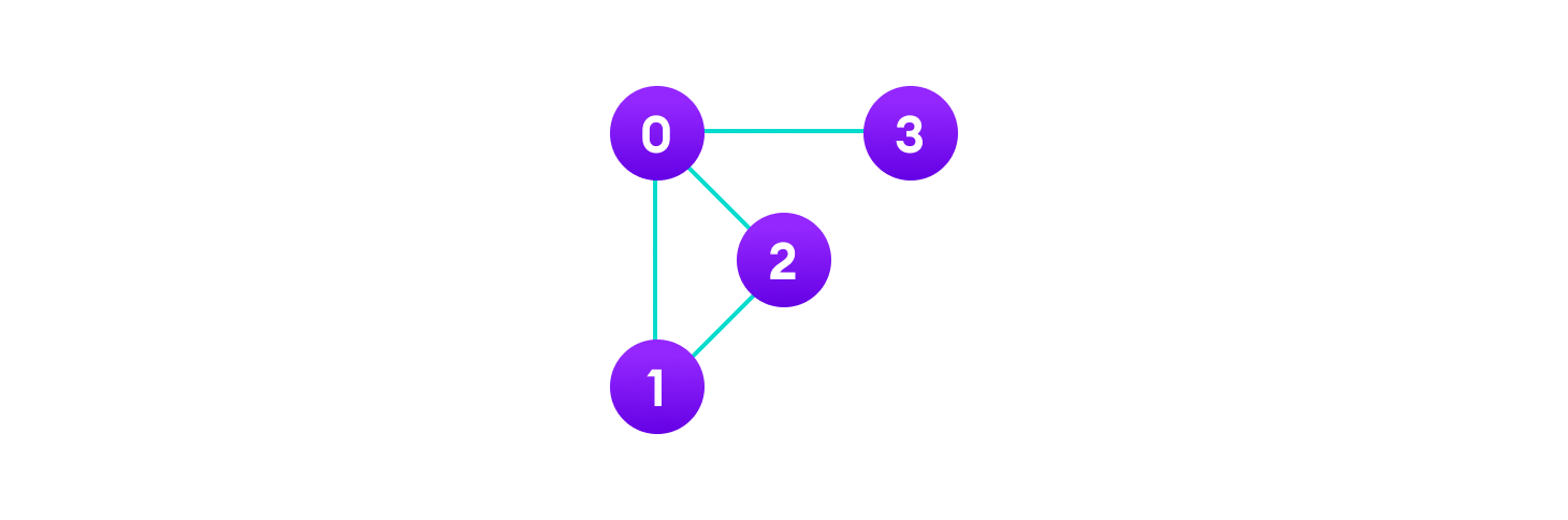
Vertices and edges

In the graph,

V = {0, 1, 2, 3}
E = {(0,1), (0,2), (0,3), (1,2)}
G = {V, E}

---

Graph Terminology

• Adjacency: A vertex is said to be adjacent to another vertex if there is an edge connecting them. Vertices 2 and 3 are not adjacent because there is no edge between them.

• Path: A sequence of edges that allows you to go from vertex A to vertex B is called a path. 0-1, 1-2 and 0-2 are paths from vertex 0 to vertex 2.

• Directed Graph: A graph in which an edge (u,v) doesn't necessarily mean that there is an edge (v, u) as well. The edges in such a graph are represented by arrows to show the direction of the edge.

---

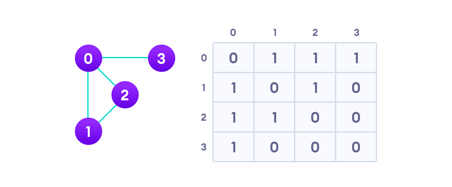
Graph Representation

Graphs are commonly represented in two ways:

1. Adjacency Matrix

An adjacency matrix is a 2D array of V x V vertices. Each row and column represent a vertex.

If any element a[i][j] has value 1, it indicates that there is an edge connecting vertex I and vertex j.

The adjacency matrix for the graph we created above is

Heap:

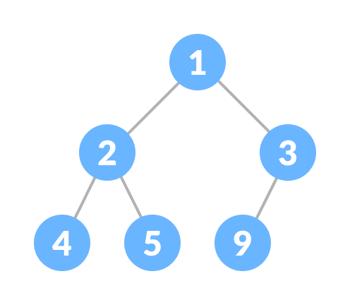
A heap data structure is a complete binary tree satisfying the heap property where any node

is always greater than its child node/s and the root node's key is the largest among all other nodes. This property is also known as the maximum heap property.

is always smaller than the child node/s and the root node's key is smaller than all other nodes. This property is also known as the mini heap property.

Min-heap

This type of data structure is also called a binary heap.

---

Heap Operations

Some of the important operations performed on a heap are described below along with their algorithms.

Heapify

Heapify is the process of creating a heap data structure from a binary tree. It is used to create a Min-Heap or a Max-Heap.

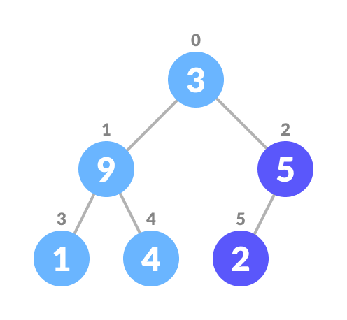
1. Let the input array be

   

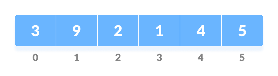
   Initial Array

2. Create a complete binary tree from the array

   

   Complete binary tree

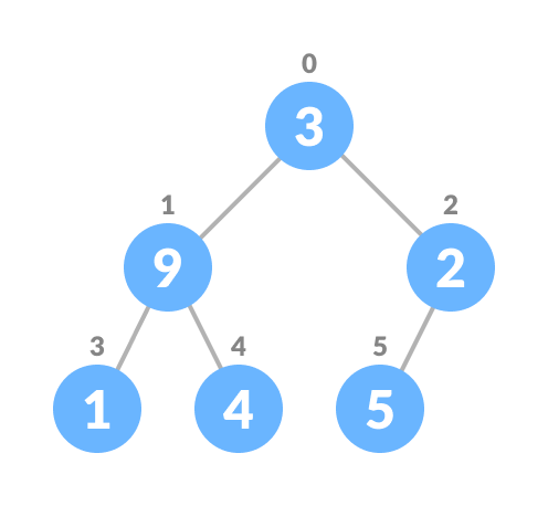
3. Start from the first index of non-leaf node whose index is given by n/2 - 1.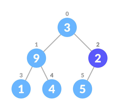

   

   Start from the first leaf node

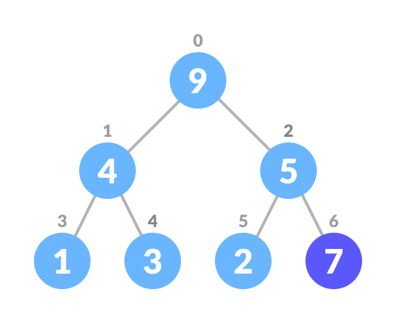
4. Set current element I to largest.

   The index of the left child is given by 2i + 1 and the right child is given by 2i + 2. If the left child is greater than the current element (ie the element at the ith index), set the left child's index to the largest. If a right child is greater than the largest element, set rightChildIndex to largest.

   Replace the current element with the largest

   

   Swap if necessary

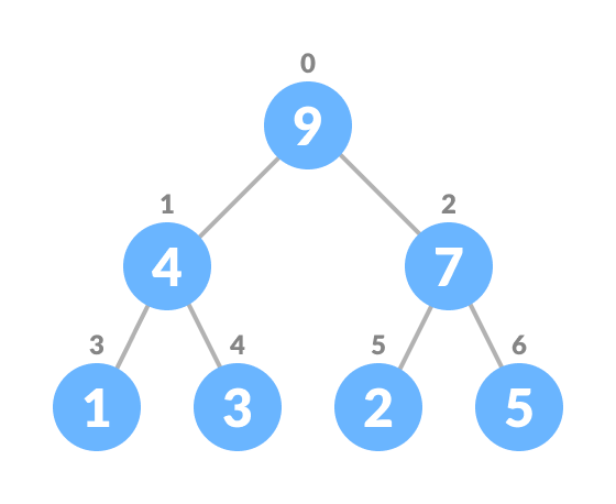
5. Repeat steps 3-7 until the subtrees are also heapified.

Algorithm

Heapify(array, size, i)
  set i as largest
  leftChild = 2i + 1
  rightChild = 2i + 2

  if leftChild > array[largest]
    set leftChildIndex as largest
  if rightChild > array[largest]
    set rightChildIndex as largest

  swap array[i] and array[largest]

To create a Max-Heap:

MaxHeap(array, size)
  loop from the first index of non-leaf node down to zero
    call heapify

For Min-Heap, both leftChild and rightChild must be larger than the parent for all nodes.

---

Insert Element into Heap

Algorithm for insertion in Max Heap

If there is no node, 
  create a newNode.
else (a node is already present)
  insert the newNode at the end (last node from left to right.)

heapify the array

1. Insert the new element at the end of the tree.

   

   Insert at the end

2. Heapify the tree.

Heapify the array

For Min Heap, the above algorithm is modified so that parentNode is always smaller than newNode.

---

Delete Element from Heap

Algorithm for deletion in Max Heap

If nodeToBeDeleted is the leafNode
  remove the node
Else swap nodeToBeDeleted with the lastLeafNode
  remove noteToBeDeleted

heapify the array

1. Select the element to be deleted.

   

   Select the element to be deleted

2. Swap it with the last element.

   

   Swap with the last element

3. Remove the last element.

   

   Remove the last element

4. Heapify the tree.

Heapify the array

For Min Heap, the above algorithm is modified so that both childnodes are smaller than the current node.

---

Peek (Find max/min)

Peek operation returns the maximum element from Max Heap or minimum element from Min Heap without deleting the node.

For both Max heap and Min Heap

return rootNode

---

Extract-Max/Min

Extract-Max returns the node with maximum value after removing it from a Max Heap whereas Extract-Min returns the node with minimum after removing it from Min Heap.

# Max-Heap data structure in Python

def heapify(arr, n, i):
    largest = i
    l = 2 * i + 1
    r = 2 * i + 2 

    if l < n and arr[i] < arr[l]:
        largest = l

    if r < n and arr[largest] < arr[r]:
        largest = r

    if largest != i:
        arr[i],arr[largest] = arr[largest],arr[i]
        heapify(arr, n, largest)

def insert(array, newNum):
    size = len(array)
    if size == 0:
        array.append(newNum)
    else:
        array.append(newNum);
        for i in range((size//2)-1, -1, -1):
            heapify(array, size, i)

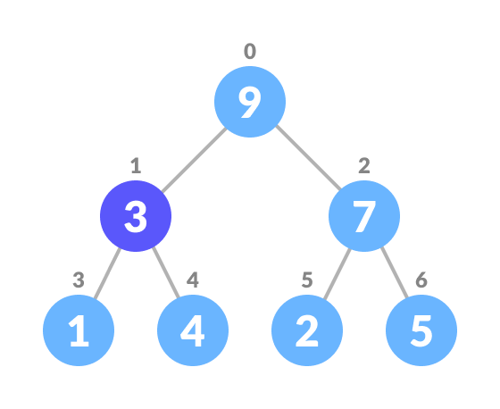
def deleteNode(array, num):
    size = len(array)
    i = 0
    for i in range(0, size):
        if num == array[i]:
            break

    array[i], array[size-1] = array[size-1], array[i]

    array.remove(num)

    for i in range((len(array)//2)-1, -1, -1):
        heapify(array, len(array), i)

arr = []

insert(arr, 3)
insert(arr, 4)
insert(arr, 9)
insert(arr, 5)
insert(arr, 2)

print ("Max-Heap array: " + str(arr))

deleteNode(arr, 4)
print("After deleting an element: " + str(arr))

---

Heap Data Structure Applications

• Heap is used while implementing a priority queue.

• Dijkstra's Algorithm

• Heap Sort

Hash Table

The Hash table data structure stores elements in key-value pairs where

Key- A unique integer used to index values

Value - The data associated with the keys.

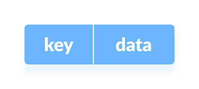
Key and value in a hash table

Hashing (Hash Function)

In a hash table, a new index is processed using the keys. And, the element corresponding to that key is stored in the index. This process is called hashing

Let k be a key and h(x) be a hash function.

Here, h(k) will give us a new index to store the element linked with k.

---

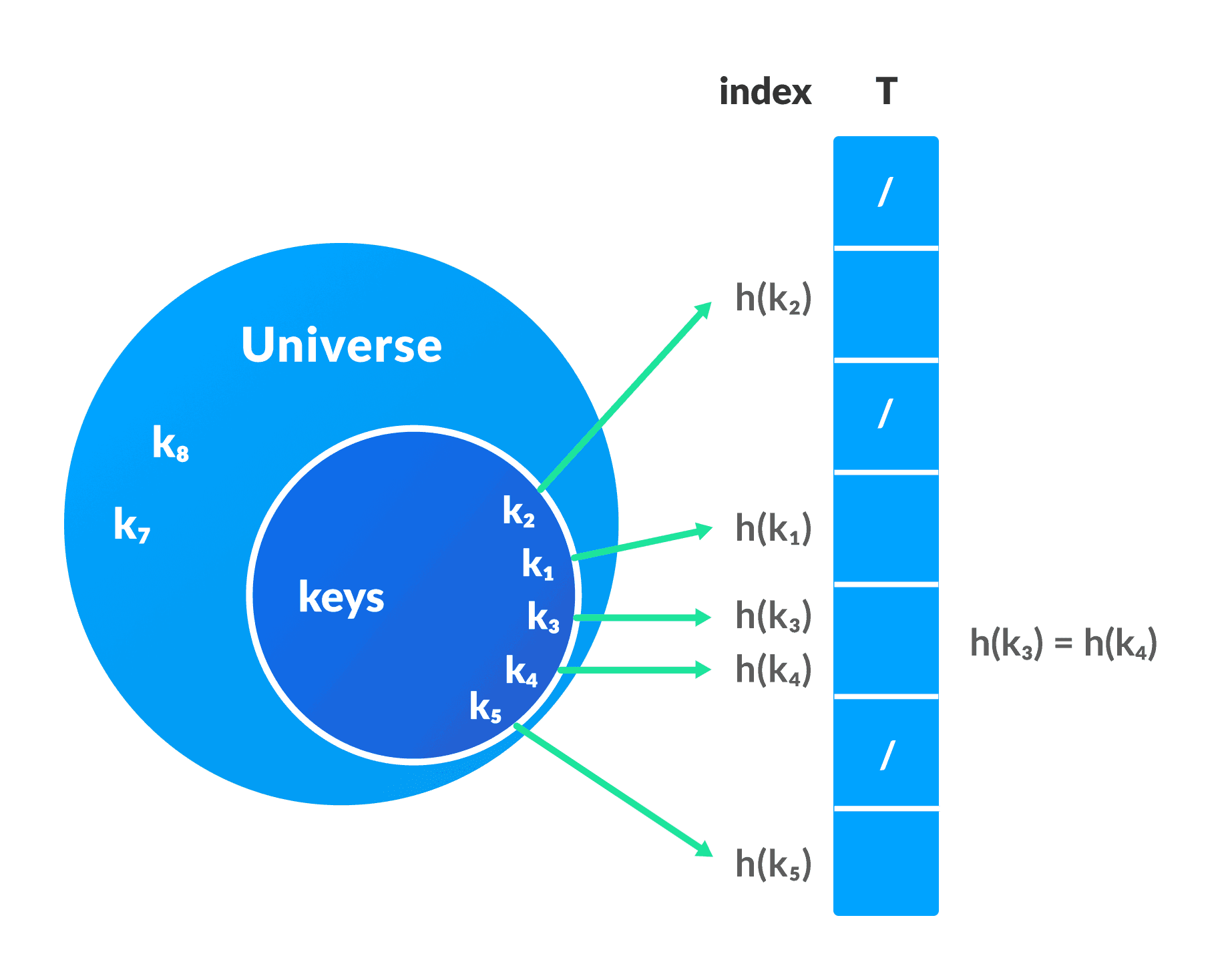
Hash Collision

When the hash function generates the same index for multiple keys, there will be a conflict (what value to be stored in that index). This is called a hash collision

We can resolve the hash collision using one of the following techniques.

• Collision resolution by chaining

• Open Addressing: Linear/Quadratic Probing and Double Hashing

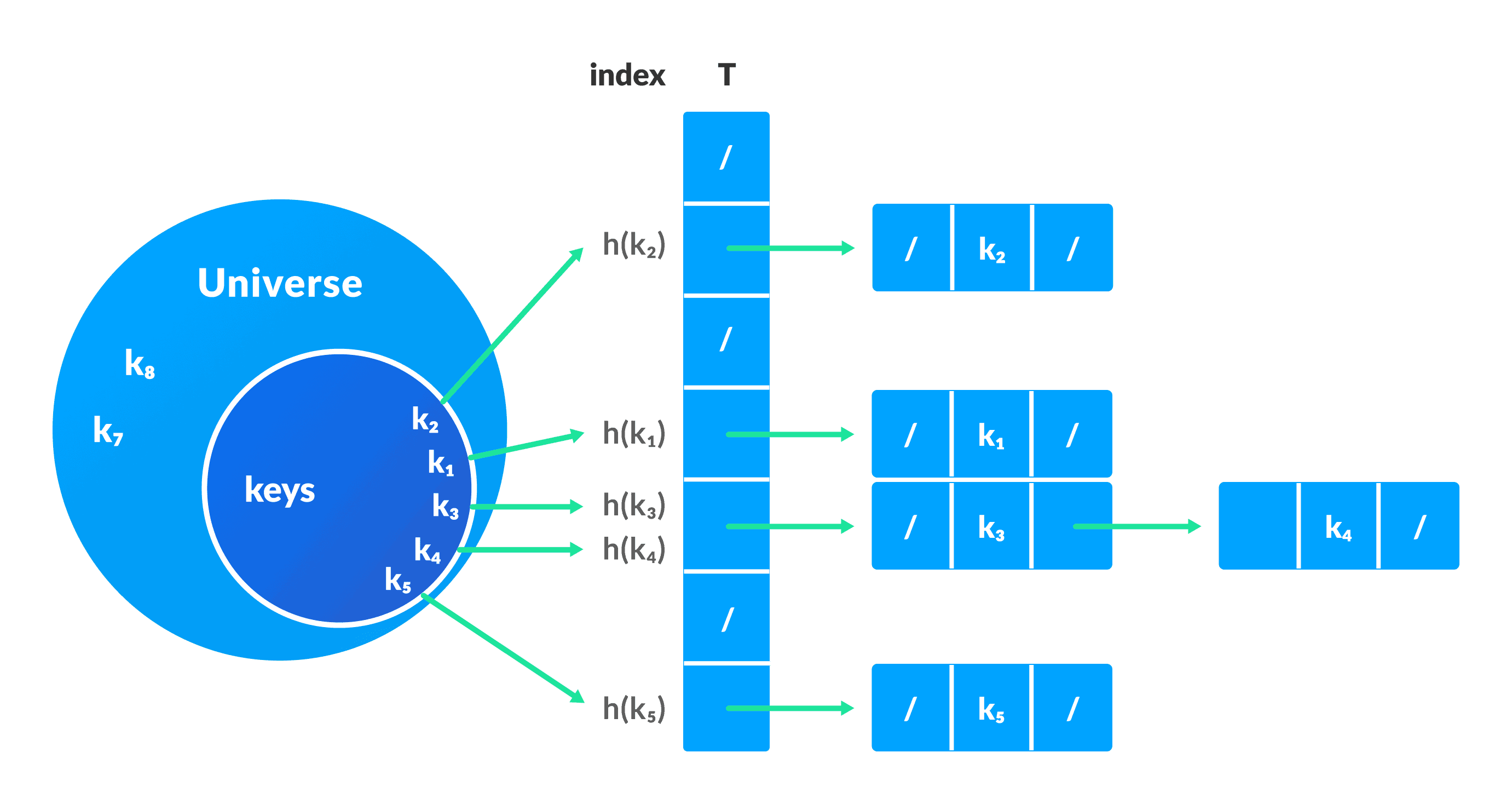
1. Collision resolution by chaining

In chaining, if a hash function produces a single index for multiple elements, these elements are stored in a single index by using a doubly-linked list.

If j is a slot for multiple elements, it contains a pointer to the head of the list of elements. If the element is absent, j contains NIL.

Collision Resolution using chaining

Pseudocode for operations

chainedHashSearch(T, k)
  return T[h(k)]
chainedHashInsert(T, x)
  T[h(x.key)] = x //insert at the head
chainedHashDelete(T, x)
  T[h(x.key)] = NIL

---

2. Open Addressing

Unlike chaining, open addressing doesn't store multiple elements into the same slot. Here, each slot is either filled with a single key or left NIL.

Different techniques used in open addressing are:

i. Linear Probing

In linear probing, a collision is resolved by checking the next slot.

h(k, i) = (h′(k) + i) mod m

where

i = {0, 1,….}

h(k) is the new hash function

If a collision occurs at h(k, 0), h(k, 1) is checked. Thus, the value of i is linearly increased

The problem with linear probing is that a cluster of adjacent slots are filled. When inserting a new element, the entire cluster must be traversed. This adds to the time required to perform operations on the hash table.

ii.Quadratic Probing

It works similarly to linear probing but increases the spacing between slots (more than one) by using the following relationship.

h(k, i) = (h′(k) + c1i + c2i2) mod m

where,

c1 and c2 are positive auxiliary constants,

i = {0, 1,….}

iii. Double Hashing

If a collision occurs after applying the hash function h(k), another hash function is calculated to find the next slot.

h(k, i) = (h1(k) + ih2(k)) mod m

Good hash functions

A good hash function may not completely prevent collisions, but it can reduce the number of collisions.

Here, we will look at different methods to find a good hash function

1. Method of division

If k is the key and m is the size of the hash table, the hash function h() is computed as:

h(k) = k mod m

For example, if the size of the hash table is 10 and k = 112 then h(k) = 112 mod 10 = 2. The value of m must not be a power of 2. This is because the binary format is powers of 2. 10, 100, 1000,... When we find k mod m, we always get lower-order p-bits.

if m = 22, k = 17, then h(k) = 17 mod 22 = 10001 mod 100 = 01
if m = 23, k = 17, then h(k) = 17 mod 22 = 10001 mod 100 = 001
if m = 24, k = 17, then h(k) = 17 mod 22 = 10001 mod 100 = 0001
if m = 2p, then h(k) = p lower bits of m

2. Multiplication Method

h(k) = ⌊m(kA mod 1)⌋

where,

kA mod 1 gives the partial component kA,

⌊ ⌋ gives the ground value

A is any constant. The value of A is between 0 and 1. But, ≈ (√5-1)/2 suggested by Knuth is the correct choice.

3. Universal Hashing

In Universal hashing, the hash function is chosen at random independent of keys.

# Python program to demonstrate working of HashTable 

hashTable = [[],] * 10

def checkPrime(n):
    if n == 1 or n == 0:
        return 0

    for i in range(2, n//2):
        if n % i == 0:
            return 0

    return 1


def getPrime(n):
    if n % 2 == 0:
        n = n + 1

    while not checkPrime(n):
        n += 2

    return n


def hashFunction(key):
    capacity = getPrime(10)
    return key % capacity


def insertData(key, data):
    index = hashFunction(key)
    hashTable[index] = [key, data]

def removeData(key):
    index = hashFunction(key)
    hashTable[index] = 0

insertData(123, "apple")
insertData(432, "mango")
insertData(213, "banana")
insertData(654, "guava")

print(hashTable)

removeData(123)

print(hashTable)

---

Applications of Hash Table

Hash tables are implemented where

• constant time lookup and insertion is required

• cryptographic applications

• indexing data is required